Optimizing the whole pipeline, not just the model: real-time YOLOv8 on Jetson
The earlier posts in this series used MobileNetV2 — a classifier, light enough that a 100 Hz loop had 6 ms of slack. Useful for isolating the clock governor, but not what a robot actually runs. Robots run detection: where is the object, not just what is it. So this finale takes the model robots actually use for vision — YOLOv8s — and asks a different question. Not “why is it slow,” but “where does the time actually go across the whole pipeline, and how far can I cut it?”
One thing to set straight up front, because the earlier posts were strict about it: this post is not a periodic real-time validation. Parts 1–3 ran a 100 Hz loop for 100k cycles and reported p99.99 and deadline misses. This one is a per-stage latency analysis — p50 over a few hundred iterations, to see where the cost lives and what optimizing each stage buys. Tail behavior under a periodic deadline is a separate test I haven’t run on this pipeline. Keep that in mind when you read “8 ms”: it’s a median pipeline latency, not a guaranteed worst-case.
The short version: a naive full pipeline is 27 ms p50. Optimized, about 8 ms. And the most interesting part wasn’t the model at all.
The naive pipeline
A detection cycle is three stages, not one:
- preprocess — take a 640×640 frame, normalize to [0,1], convert HWC→CHW, cast to float32
- inference — the YOLOv8s forward pass
- postprocess — decode ~8400 raw boxes, filter by confidence, run NMS
Written the obvious way — numpy preprocess, ONNX Runtime on the CUDA provider, NMS on CPU — here is where the time goes (640×640, p50):
| stage | latency |
|---|---|
| preprocess | 2.57 ms |
| inference | 23.98 ms |
| postprocess (NMS) | 0.70 ms |
| end-to-end | 27.25 ms |
This isn’t a strawman — it’s what you get following the tutorials. And note the first lie already: if you benchmark inference only, you report 24 ms. The thing a robot actually waits on is 27 ms. Inference-only numbers undercount the real loop, the same way back-to-back numbers undercounted the periodic loop in Part 1.
27 ms is ~37 FPS. Fine for a 30 Hz camera, nothing to spare. Let’s optimize.
Optimizing each stage
Inference: the backend decides. The 24 ms is ONNX Runtime’s CUDA provider running the model op by op. TensorRT compiles the graph ahead of time, fuses layers, and runs in FP16. Same model, same board:
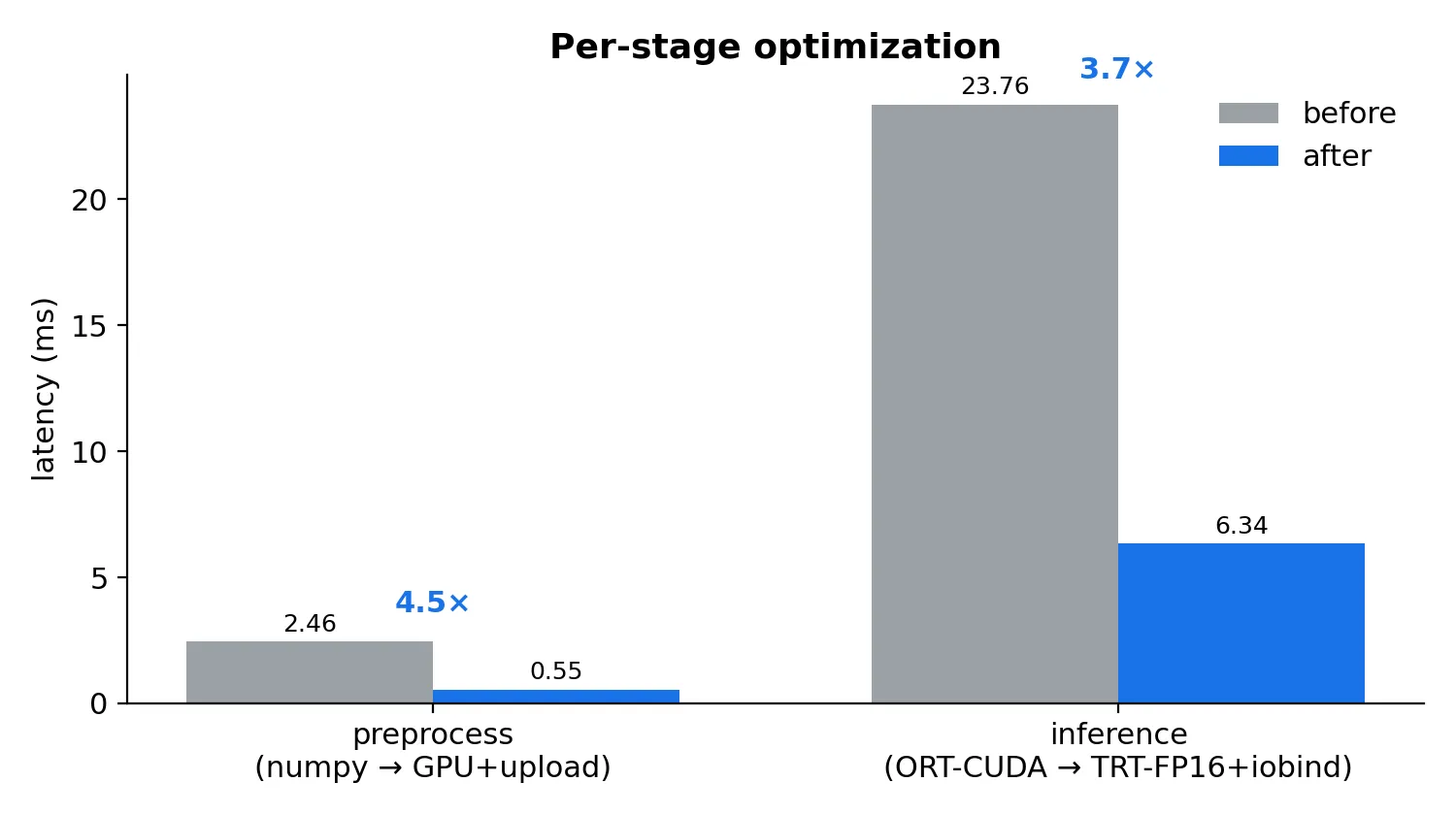
ORT-CUDA 23.76 ms → TensorRT-FP16 6.34 ms. A 3.7× cut, from changing nothing but the execution backend. For a heavy model on the edge, the backend is the difference between real-time and not.
Preprocess: it moves to the GPU. Once inference drops to 6 ms, the 2.5 ms numpy preprocess is no longer a rounding error — it’s a quarter of the budget. Breaking it down, the cost is the float32 cast/normalize (1.45 ms) and the contiguous copy (1.12 ms): a single CPU thread touching 1.2M floats. The fix is to not do it on the CPU. Upload the uint8 frame (a quarter the bytes of float32) and cast/normalize/transpose on the GPU: 2.46 ms → 0.55 ms, 4.5×.
Connecting them without a round trip. GPU preprocess only helps if the
result doesn’t bounce back to the CPU before inference. ONNX Runtime’s
io_binding lets you hand inference a GPU pointer directly — the preprocessed
tensor stays on the GPU, inference reads it in place, and the output stays on
the GPU too. No per-frame host↔device copies. This shaved another ~1 ms off
inference (the input copy it was doing implicitly): TensorRT-FP16 with io_binding
runs at 6.34 ms, and its output is already on the GPU for postprocess to pick up.
That last point — building one path where data lands on the GPU and stays there through all three stages — is the part that matters for an actual robot. It’s not three benchmarks bolted together; it’s a pipeline.
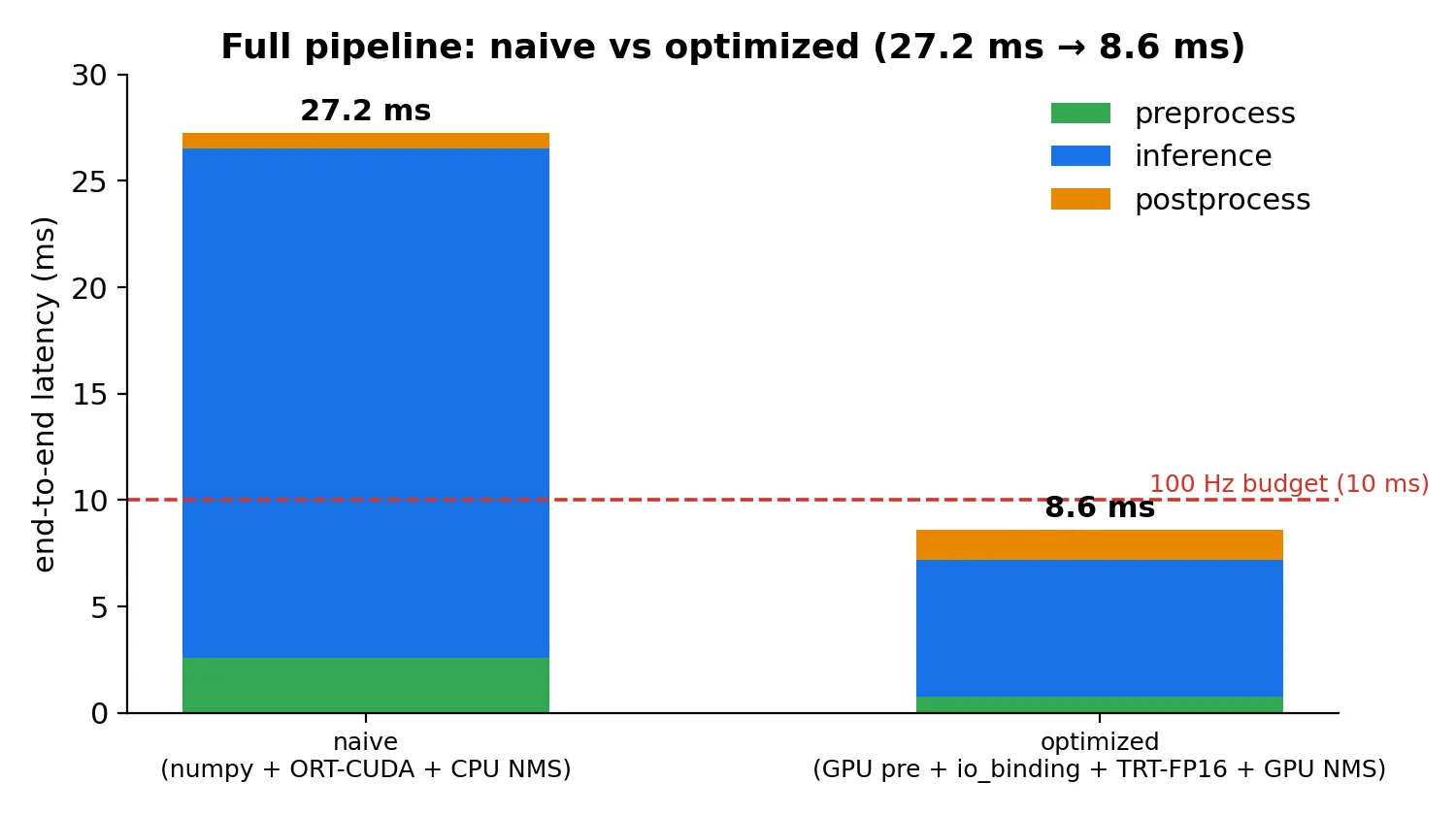
Stack it up: 27.25 ms → 8.62 ms p50, 3.2×. The median now sits under 10 ms — though whether it holds a 10 ms deadline across 100k cycles is the tail question I’m not answering here. I could have stopped at the stack. But the postprocess bar grew — relatively — and I wanted to know what was in it.
The reversal: in this pipeline, NMS wasn’t the cost
Everyone calls postprocess “NMS.” Non-max suppression is the famous part — the O(n²) box comparison. So I expected, with inference down to 6 ms, that NMS would be the next thing to fight.
I measured it. In this implementation, I was wrong.
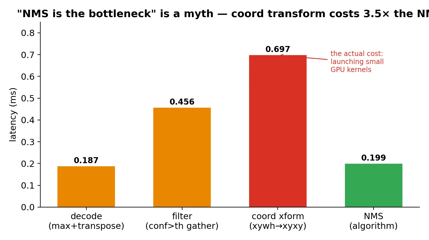
Splitting postprocess into its actual steps, on real detections:
| step | latency |
|---|---|
| decode (max over 80 classes + transpose) | 0.19 ms |
| filter (confidence threshold, gather) | 0.46 ms |
| coordinate transform (xywh→xyxy) | 0.70 ms |
| NMS (the algorithm) | 0.20 ms |
NMS is the cheapest meaningful step. The most expensive is the four lines that
convert box coordinates from center-format to corner-format — xy[:,0] = b[:,0] - b[:,2]/2 and its three siblings. Not because the math is heavy: it’s
1000-odd boxes. It’s that each line is a separate small GPU kernel launch on a
small tensor, and for small tensors the launch overhead dominates the work. Four
lines, eight strided index operations, and the launches add up to 0.7 ms — three
and a half times the NMS it’s preparing data for.
I confirmed it wasn’t NMS hiding in there: moving NMS to the CPU left the 0.7 ms untouched. The cost isn’t what is computed, it’s how many times the GPU is poked and when it’s synchronized. The step’s name (“NMS”) had nothing to do with where its time went.
This is the same lesson as Part 1, one level deeper. There, benchmarking back-to-back hid periodicity. Here, naming the stage “NMS” hid that the cost is tensor plumbing, not the algorithm. You only see it if you measure the pipeline you actually run.
One caveat I’ll state plainly: this is about my postprocess code. A fused kernel, a TensorRT NMS plugin, or Ultralytics’ own postprocess would distribute the cost differently — the coordinate transform might vanish into a fused op. The claim isn’t “NMS is never the bottleneck.” It’s narrower and, I think, more useful: the stage’s name told me nothing about where its time went, and only measuring the steps did.
When “just use the GPU” is wrong
There’s a corollary. My optimized pipeline ran NMS on the GPU, because the rest of the pipeline was already there and moving data off felt wasteful. But NMS has a fixed GPU launch overhead, and at the box counts real scenes produce, that overhead is the whole cost. Sweep the number of boxes into NMS:
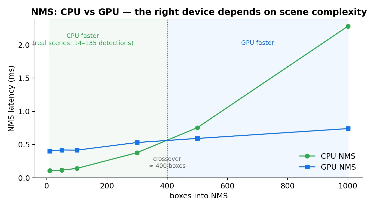
CPU NMS is faster up to ~400 boxes; GPU NMS is faster beyond. Real images, as we’ll see, produce 14–135 detections — squarely in CPU territory. In the synthetic sweep, running NMS on the CPU here costs ~0.2 ms versus the GPU’s ~1.2 ms in-pipeline. “Optimized” does not mean “everything on the GPU.” The right device depends on how many boxes the scene actually contains, and for detection on real scenes, that’s few.
So there are two numbers, and they shouldn’t be conflated. In the synthetic box-count benchmark, swapping to CPU NMS pulls the optimized pipeline to ~7.7 ms p50. On the 15 real images below — measured end to end, GPU NMS as-built — it’s ~8.9 ms p50, and ~8.9 with CPU NMS too (the CPU/GPU NMS gap is small at these box counts and partly hidden by the rest of the pipeline). Treat 7.7 ms as the synthetic best-case and ~8.9 ms as what the real-image runs actually produced.
Does this hold on real images?
The box-count sweep above is synthetic — I injected N boxes to control scene complexity. Real detections cluster and overlap differently. So I ran the optimized pipeline on 15 COCO val images spanning empty-ish scenes to crowds, with real detections and real NMS:
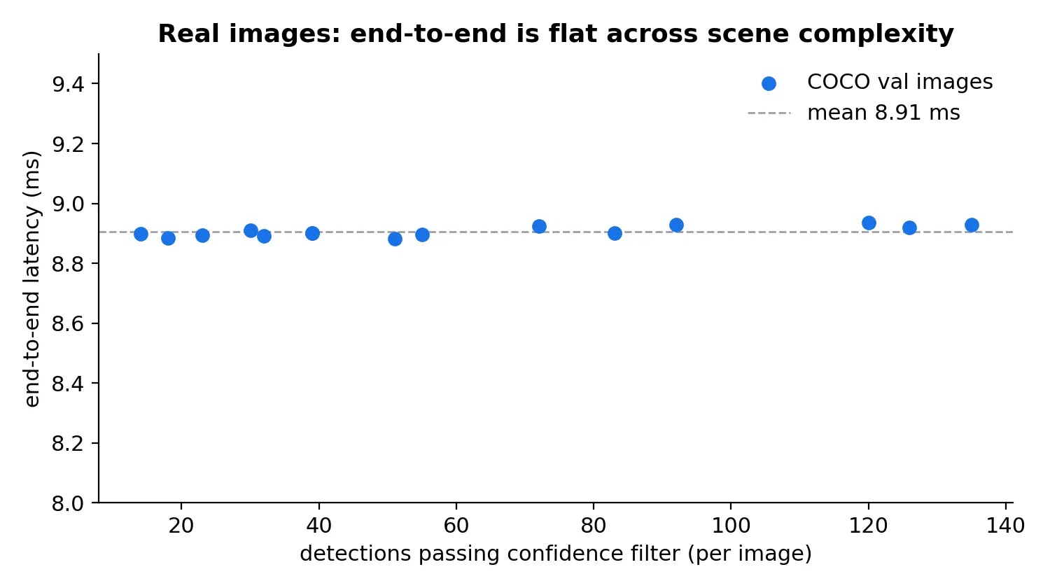
End-to-end sits at 8.9 ms (GPU NMS build) regardless of whether the image has 14 detections or 135. Preprocess (0.75 ms) and inference (6.42 ms) are fixed — they don’t care what’s in the frame. And postprocess, across that 10× range in detection count, is flat too: in this regime the fixed per-stage overheads dominate, not the box count. The synthetic sweep shows box count can matter, but only past a few hundred — well beyond what these scenes produce.
So the real-image numbers land on the synthetic curve, at the low-box end where real scenes live. The controlled sweep wasn’t a fiction; it just exercised a range most detection scenes never reach.
Where this lands, and what it isn’t
Naive full pipeline: 27.2 ms p50. Optimized — TensorRT-FP16, GPU preprocess, zero-copy io_binding: ~8.9 ms p50 on real images (and ~7.7 ms in the synthetic CPU-NMS best case). About 3–3.5×, on a Jetson Orin Nano Super.
Two things worth saying plainly. First, the headline of the whole series holds in its strongest form here: optimizing the model alone is a lie. Cutting inference 3.7× only cut end-to-end 2.4× until I went after preprocess and the data path; and the postprocess bottleneck wasn’t even the stage everyone names. The pipeline is the unit of optimization, not the model.
Second, the scope — and here this post is weaker than the three before it, so I’ll be exact. This is a p50 pipeline-latency analysis, not a periodic real-time validation. Parts 1–3 ran a 100 Hz loop for 100k cycles and reported p99.99 and deadline misses; this post does not. A median under 10 ms is not a held deadline — the tail and the miss rate under a periodic schedule are unmeasured here, and they’re what actually decide real-time. On top of that: one model, one board, pre-decoded frames, a cool room. A real robot adds what I did not measure here: a camera and its ISP/decode path ahead of preprocess, and — the big one — other work contending for the same GPU (a second model, a tracker, the rest of the stack). Single- stream, single-model latency is the floor, not the number you’ll see under a full robot load. Those are real, and they’re outside this post.
But the pipeline is real, it’s built, and it runs. Code, the per-stage harness, the box-count sweep, and the COCO anchor measurements are in the repo: github.com/dankang21/jetson-latency-lab.
That closes the series. Four posts, one board, one question asked four ways: the number you benchmark is rarely the number you run. Back-to-back hid periodicity; inference-only hid the pipeline; “NMS” hid the plumbing. Measure the loop you actually deploy.