Back-to-back benchmarks lie: a 100,000-cycle study of periodic 100 Hz inference on Jetson Orin Nano Super
The number everyone quotes is the number you will never see in production.
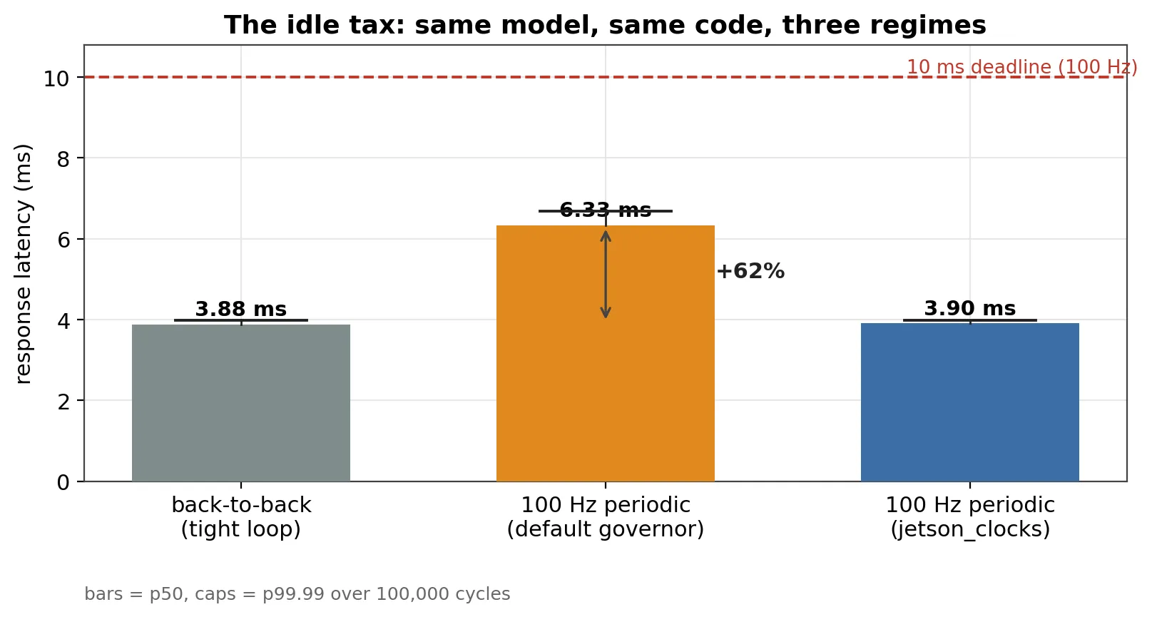
I ran MobileNetV2 on a Jetson Orin Nano Super two ways. Back to back, as fast as the GPU will go, it serves an inference in 3.88 ms. Driven at a fixed 100 Hz — the way an actual control loop runs it — the same model, same code, same board, takes 6.33 ms. That is a 62% increase, and none of it is the scheduler’s fault. The cause is the GPU clocking itself down in the idle gap between cycles, and it disappears completely the moment you lock the clocks.
This post is the measurement, the method that makes the claim defensible, and the one-line fix.
Why periodic, and why the tail
A perception or policy network on a robot does not run in a tight loop. It runs on a clock: every 10 ms a new frame arrives, you infer, you act, you wait for the next frame. The 6 ms you are not inferring is not free time — it is time the hardware spends deciding you are idle.
And the metric that matters is not the mean. A control loop that meets its deadline 99.9% of the time and blows it once a second is broken. So the question is not “how fast on average” but “what is the worst case over a long run, and does it ever miss the deadline.” I measured 100,000 cycles. p99.99 is the worst 0.01% — about the 10 slowest cycles out of a hundred thousand.
Test bed
| Board | Jetson Orin Nano Super 8 GB |
| Power | MAXN_SUPER |
| Kernel | PREEMPT_RT |
| Runtime | ONNX Runtime 1.23.0, CUDA EP (PyTorch 2.9.1 / CUDA 12.6 / TensorRT 10.3.0 stack) |
| Model | MobileNetV2-12, ONNX, input 1×3×224×224 |
| Loop | 100 Hz (10 ms period), 100,000 cycles, 2,000 warmup |
The inference path is single-threaded ORT (intra=inter=1), graph optimization
ENABLE_ALL, a fixed seed-42 dummy input. MobileNetV2 latency is
data-independent, so a fixed random tensor measures the same thing a real frame
would.
The lie: back to back
The standard way to benchmark inference is a tight loop — call, time, call again, no waiting. Here is that number, 100,000 iterations:
mean     = 3.882 ms
std      = 0.011 ms
p99.99   = 3.978 ms
max      = 4.205 ms
misses   = 0 / 100000   (10 ms deadline)
This is a beautiful result. Sub-4 ms at p99.99, jitter measured in single-digit microseconds, dead flat. If I published here, I would have a “Jetson does 100 Hz with 60% margin to spare” headline. It would also be wrong, because the loop that produced it is not a loop any robot runs. The GPU never went idle, so it never clocked down. The benchmark accidentally measured the best case and called it the result.
Measuring it the way it deploys
To measure the regime that ships, the loop has to be periodic, and the harness itself must not be a source of jitter — otherwise you cannot tell the system’s latency from your own. Three things make the measurement trustworthy:
- Absolute-time release. The period is held with
clock_nanosleep(CLOCK_MONOTONIC, TIMER_ABSTIME)against a fixed schedule (release_n = start + n·period). A late wake-up in one cycle does not push the next — error does not accumulate, unlike relativesleep(). - The harness runs real-time.
SCHED_FIFOpriority 80, pinned to a dedicated core, withmlockallso there are no page faults on the hot path. - Per-cycle decomposition. Every cycle records three quantities, not one:
| quantity | definition | blames |
|---|---|---|
release_jitter | wake-up − scheduled release | scheduler / IRQ latency |
compute | inference done − wake-up | GPU + framework |
response | inference done − scheduled release | end-to-end, vs deadline |
That third decomposition is the whole game. Without it you see “the tail got worse” and you guess. With it you can name the layer.
The result: the 62% idle tax
Same model, same inference code, now driven at 100 Hz with the default governor:
response  p50 = 6.333 ms   p99 = 6.610 ms   p99.99 = 6.680 ms   max = 6.726 ms
misses    = 0 / 100000
The deadline is still met — 6.7 ms < 10 ms, zero misses. But the loop is 62% slower than the back-to-back number, and it is slower consistently: p50 to p99.99 spans only 0.35 ms. This is not occasional spikes. Every single cycle pays the tax.
Whodunit: not the scheduler
Here is where the decomposition pays off. Of that 6.33 ms response time:
compute  p50 = 6306.6 us   p99.99 = 6655.0 us
jitter   p50 =   24.8 us   p99.99 =   45.0 us
99.6% of the response time is GPU compute. Scheduling jitter is 45 µs at p99.99 —
0.4% of the budget, and exactly what you want from a PREEMPT_RT kernel. So the
2.4 ms the periodic loop added over the back-to-back baseline is entirely in
the GPU, not in the kernel, not in wake-up latency, not in my harness.
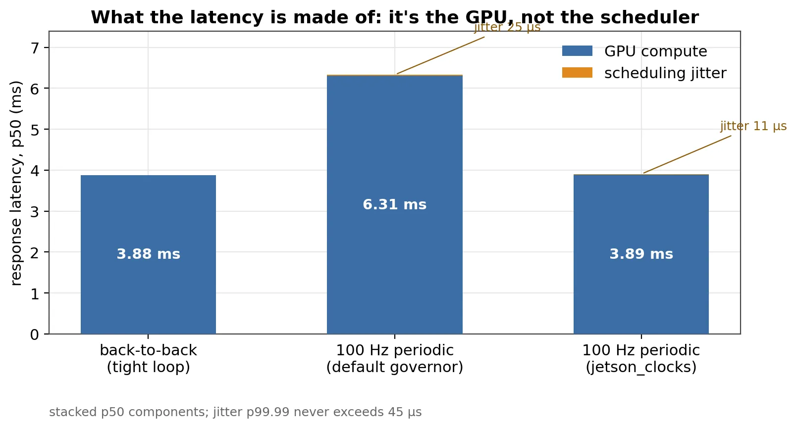
This is the part that surprises people. The instinct on a real-time board is to suspect the scheduler — the kernel, preemption, IRQ latency. The data says the kernel is innocent. The model is running slower because the GPU, seeing ~6 ms of idle every cycle, scales its frequency down and starts each inference cold.
Confirming cause: lock the clocks
If dynamic frequency scaling is the cause, freezing the clocks should erase the
effect. jetson_clocks pins CPU/GPU/EMC to maximum. Same periodic 100 Hz loop,
clocks locked:
response  p50 = 3.905 ms   p99 = 3.925 ms   p99.99 = 3.982 ms   max = 4.017 ms
compute   p50 = 3893.6 us  p99.99 = 3959.0 us
jitter    p50 =   11.0 us  p99.99 =   22.9 us
misses    = 0 / 100000
Compute returns to 3893.6 µs — within 0.3% of the back-to-back 3882 µs. The entire periodic penalty is gone. As a bonus, jitter halved too (45 → 22.9 µs): locking clocks stabilizes wake-up latency as well.
The three points side by side:
| condition | response p50 | response p99.99 | compute p50 | jitter p99.99 |
|---|---|---|---|---|
| back-to-back (tight loop) | 3.882 | 3.978 | — | — |
| 100 Hz periodic, default governor | 6.333 | 6.680 | 6306.6 µs | 45.0 µs |
100 Hz periodic, jetson_clocks | 3.905 | 3.982 | 3893.6 µs | 22.9 µs |
Locked, the loop is not just fast, it is deterministic: a 65 µs spread from p50 to p99.99 across 100,000 cycles, max 4.017 ms, zero misses. That is the kind of number a control engineer can budget against.
The takeaway
Two things, both practical:
- Benchmark in the regime you deploy. A back-to-back latency number for a model you will run periodically is not conservative — it is optimistic by the exact amount of the DVFS idle tax. Here that was 62%. Drive your benchmark at the real period.
- For periodic edge inference, pin the clocks. On this board,
jetson_clocksconverted a 62% penalty into deterministic baseline latency for free. The trade is power and heat for predictability — usually the right trade on a robot that has a deadline. (Whether locked clocks hold up under thermal load over a long run is the next question; that is part 2.)
Scope
One board, one model, one kernel build. These numbers describe this system, not Jetson in general — they depend on power mode, governor, model size, and clock state, all of which are recorded in each run’s metadata so a result is self-describing. The mechanism (idle gap → DVFS downclock → cold-start inference) generalizes; the magnitude will not.
Reproduce
The harness, stress matrix, and analysis are at
jetson-latency-lab —
periodic loop with absolute-time release, SCHED_FIFO/mlockall, and the
jitter/compute/response decomposition used above.
sudo python3 -m harness.infer_bench \
  --backend onnxruntime --model models/mobilenetv2-12.onnx \
  --hz 100 --iters 100000 --cpu 5 --prio 80 \
  --label baseline --out results/baseline